This module implements a functional principal component analysis (fPCA) pipeline designed for fMRI data. The overall procedure involves the following steps:
Data Loading and Preprocessing:
The 4D fMRI image and an associated 3D binary mask are loaded. The mask extracts voxel-specific time series, and the time axis is defined based on the number of timepoints.
B-Spline Basis Construction:
A set of B-spline basis functions is generated to represent the smooth temporal dynamics. Each voxel’s time series is approximated as a linear combination of these basis functions.
Penalty Matrix Construction:
A penalty matrix is computed to ensure smoothness of the estimated coefficients. This penalty is defined via an integral that involves the product of derivatives (typically the second derivative) of the basis functions.
Regularized Spline Regression:
For every voxel, the time series is approximated by a linear expansion in the spline basis. The coefficients of this expansion are estimated by solving a regularized regression problem. A generalized cross-validation (GCV) criterion is used to select a voxel-specific regularization parameter (\(\lambda\)).
Functional Principal Component Analysis:
PCA is then performed on the coefficients matrix to identify the dominant patterns of temporal variation. Multiplying the eigenfunctions by the coefficients yields voxel-specific importance scores that are mapped back into brain images, while the product of the basis matrix with each eigenfunction generates an intensity plot showing the common (to all voxels) temporal dynamics.
Finally, for each eignfunction, voxel importance maps and intensity plot are generated and saved.
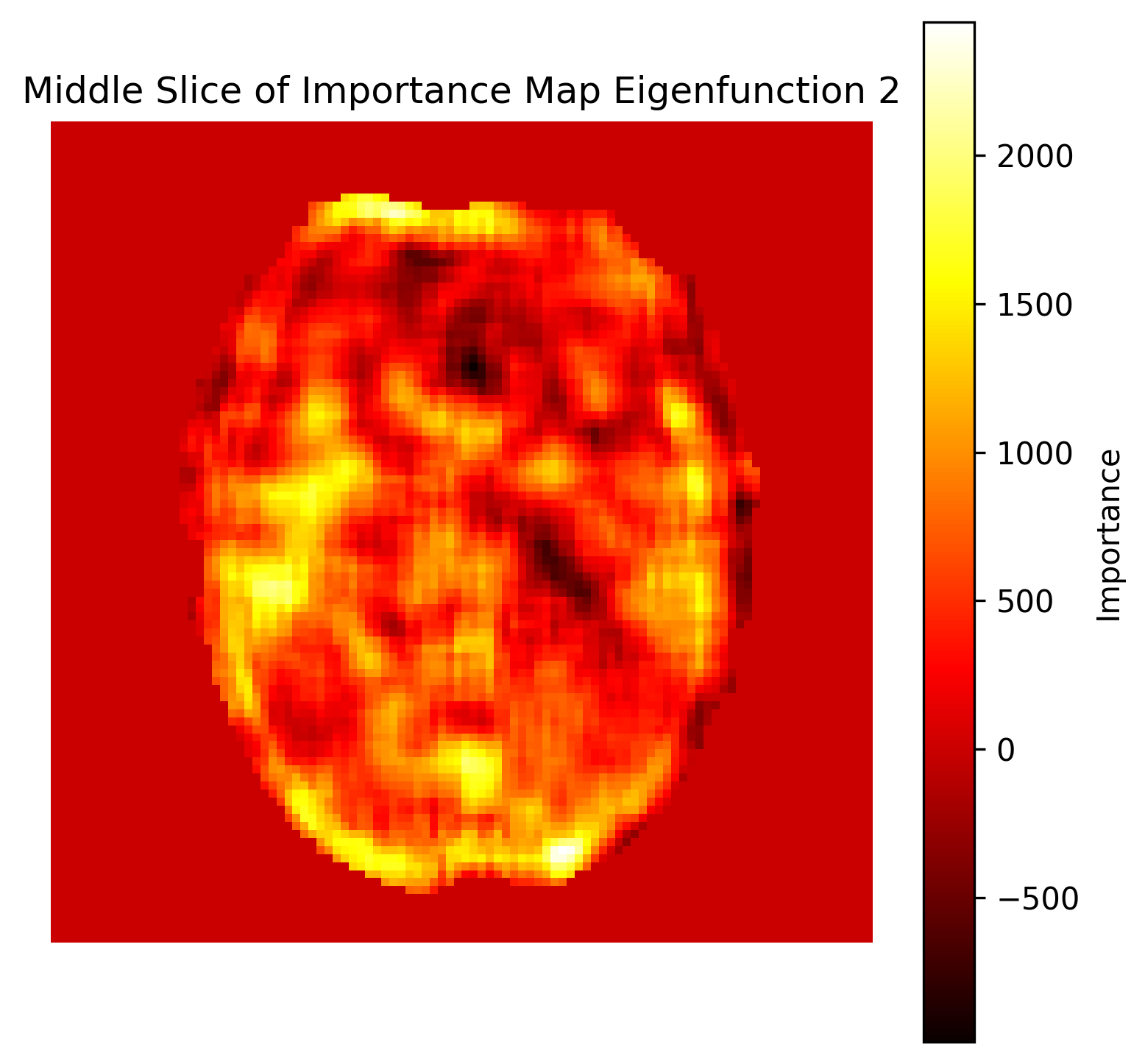
voxel importance maps:
The computed score indicates the contribution or importance of that voxel for the corresponding principal component.
Using the spatial information from the original brain mask, these voxel scores are then mapped back to a volume of the brain. This produces an importance map saved as a file with the brain’s dimensions, where each voxel’s value indicates its contribution to the fPCA component.
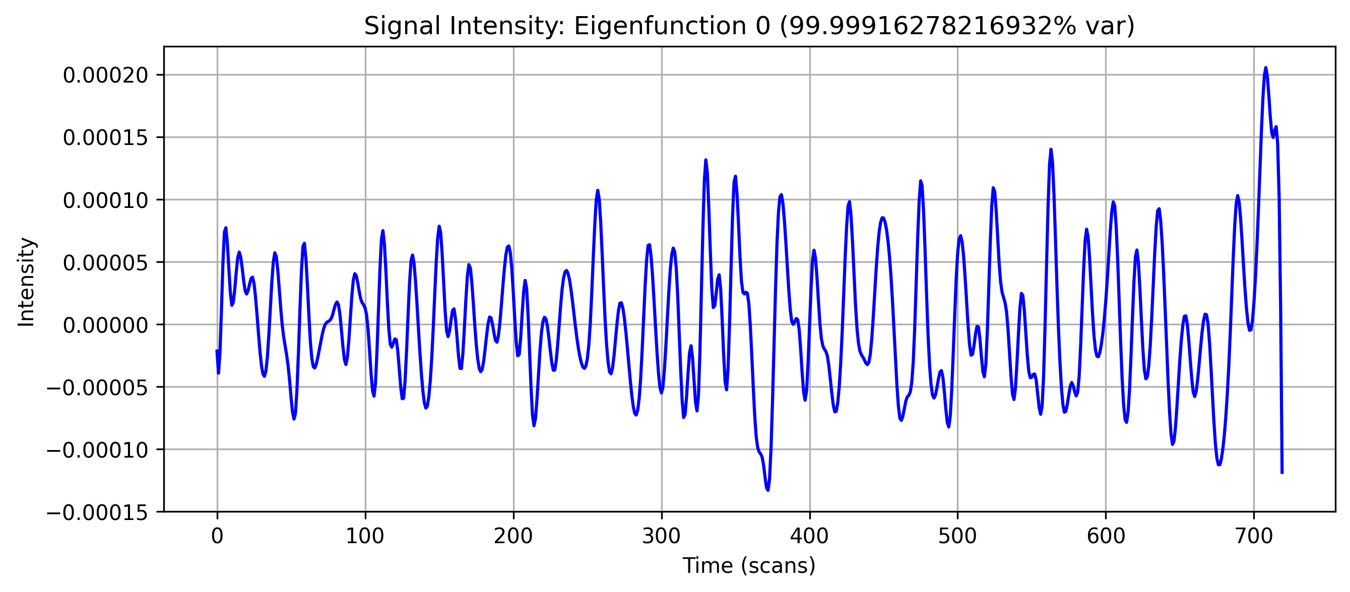
intensity plot:
The PC temporal profile values are plotted as a graph (intensity plot) that illustrates the time-course of the fPCA component across the entire brain.
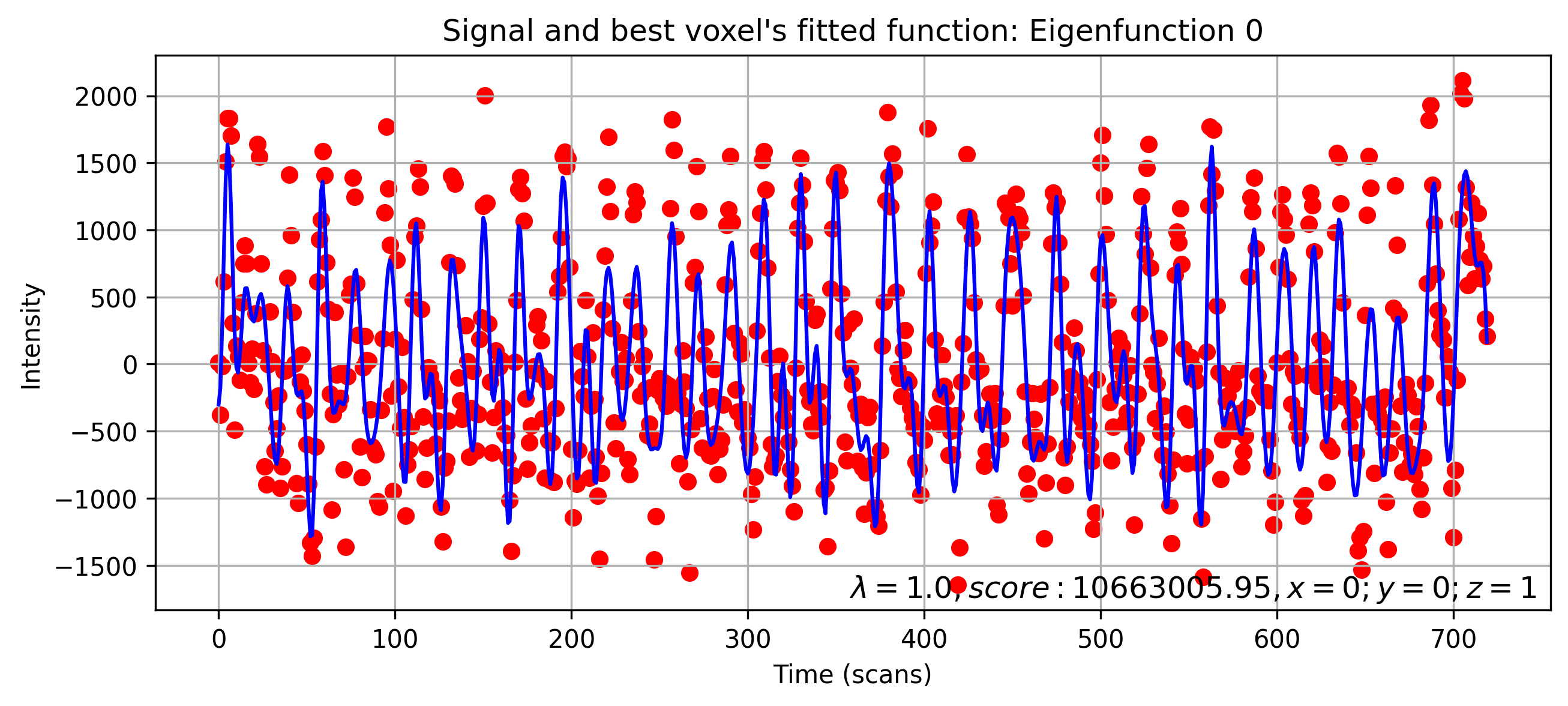
Signal Intensity for Best-Scoring Voxel
This plot illustrates the signal intensity over time for the voxel with the highest score in a given eigenfunction \(i\). The red dots represent the original fMRI signal, while the blue curve shows the corresponding fitted function based on the selected eigenfunction. The voxel is identified by its index in the 3D brain volume, and the optimal regularization parameter \(\lambda\), along with the voxel’s score and spatial coordinates \((x, y, z)\), are annotated in the figure. This visualization helps assess the quality of the functional fit at the most representative voxel for each eigenfunction.