Utility Scripts Documentation
This page provides detailed documentation for the utility scripts included in the fMRI package. These scripts are designed to streamline common preprocessing and analysis tasks.
Preprocessing Scripts
preprocess-nii-file
The preprocess-nii-file script preprocesses a single 4D fMRI NIfTI file using a 3D mask file, applying filtering and smoothing to prepare the data for later analysis. Its main purpose is to make this preprocessing step reusable — so that when running fmri-main multiple times with different parameters, you don’t need to repeat the same costly preprocessing. Instead, once the data has been preprocessed, you can run fmri-main directly on the generated outputs using the --processed flag to indicate that the preprocessing stage has already been completed.
Command Line Interface:
preprocess-nii-file --nii-file <path_to_nii> --mask-file <path_to_mask> --output-folder <output_path> [options]
Required Arguments:
--output-folder(str): Path to an existing folder where output files will be saved.
Optional Arguments:
--nii-file(str): Path to the 4D fMRI NIfTI file. If not provided, the script will prompt for input.--mask-file(str): Path to the 3D mask NIfTI file. If not provided, the script will prompt for input.--TR(float): Repetition time (TR) in seconds. If not provided, it will be extracted from the NIfTI header.--smooth_size(int): Box size of smoothing kernel (default: 5).--highpass(float): High-pass filter cutoff frequency in Hz. Filters out slow drifts below this frequency (default: 0.01).--lowpass(flpat): Low-pass filter cutoff frequency in Hz. Filters out high-frequency noise above this frequency (default: 0.08).
What the Script Does:
Loads the 4D fMRI data and 3D mask
Applies temporal filtering and spatial smoothing
Saves the filtered data as a new NIfTI file with “_filtered” suffix
Outputs the processed file to the specified output folder
Example Usage:
# Basic usage
preprocess-nii-file --nii-file /path/to/subject_bold.nii.gz \
                    --mask-file /path/to/brain_mask.nii.gz \
                    --output-folder /path/to/preprocessed_data/

# With custom parameters
preprocess-nii-file --nii-file /path/to/subject_bold.nii.gz \
                    --mask-file /path/to/brain_mask.nii.gz \
                    --output-folder /path/to/preprocessed_data/ \
                    --TR 0.75 \
                    --smooth_size 3 \
                    --highpass 0.01 \
                    --lowpass 0.08
Output:
The script creates a filtered NIfTI file in the output folder with the naming convention: <original_filename>_filtered.nii
Notes:
The output folder must exist before running the script
The script automatically handles both compressed (.nii.gz) and uncompressed (.nii) NIfTI files
Processing time depends on the size of the input data and smoothing parameters
Batch Processing Scripts
preprocess_multiple_files.sh
The preprocess_multiple_files.sh script is a Bash script designed to batch process multiple NIfTI files with their corresponding mask files. It automates the preprocessing multiple nii files.
Purpose
This script automates the preprocessing of multiple fMRI files by:
Finding all bold files in a specified input directory
Matching each bold file with its corresponding brain mask
Running the
preprocess-nii-filecommand for each valid pairOrganizing output files in a structured manner
Script Structure:
The script expects files to be named with a specific pattern:
Bold files:
<base_name>-preproc_bold.nii*Mask files:
<base_name>-brain_mask.nii.gz
Current Configuration:
INPUT_DIR="/folder/with/raw-files/"
OUTPUT_DIR="preprocessed_data"
How to Customize:
Update Input Directory: Modify the
INPUT_DIRvariable to point to your data directory:INPUT_DIR="/path/to/your/fmri/data/"
Update Output Directory: Change the
OUTPUT_DIRvariable for your preferred output location:OUTPUT_DIR="/path/to/your/preprocessed/data/"
Update Virtual Environment Path: Modify the activation path if using a different virtual environment:
source /path/to/your/venv/bin/activate
Modify Parameter Ranges:
max_parallel_samples=1 # Maximum number of parallel processes. Adjust based on system capabilities.
Usage:
# Make the script executable
chmod +x preprocess_multiple_files.sh

# Run the script
bash preprocess_multiple_files.sh
What the Script Does:
Creates the output directory if it doesn’t exist
Searches for all bold files matching the pattern
*bold*.nii*For each bold file, attempts to find the corresponding brain mask
Runs
preprocess-nii-filefor each valid file pairLogs the processing status for each file
File Organization Expected:
input_directory/
├── subject1-preproc_bold.nii.gz
├── subject1-brain_mask.nii.gz
├── subject2-preproc_bold.nii.gz
├── subject2-brain_mask.nii.gz
└── ...
Output Structure:
preprocessed_data/
├── subject1-preproc_bold_filtered.nii
├── subject2-preproc_bold_filtered.nii
└── ...
Troubleshooting:
Ensure the virtual environment path is correct
Verify that file naming conventions match the expected patterns
Check that the input directory contains both bold and mask files
Make sure the fMRI package is installed in the virtual environment
run_parameter_combinations.sh
The run_parameter_combinations.sh script performs comprehensive parameter sweeps for fMRI analysis, testing multiple combinations of parameters to find optimal settings for your data.
Purpose:
This script systematically tests different parameter combinations for fMRI analysis including:
Different derivative orders (p and u parameters)
Various threshold values
Multiple lambda ranges for regularization
Different numbers of basis functions
Both penalized and non-penalized approaches
Current Parameter Sets:
derivatives=(0 1 2)
thresholds=(1e-3 1e-6)
lambda_ranges=("0 6" "-6 0" "-6 6")
n_basis_values=(100 200 300 400)
MAX_PARALLEL=8  # Maximum number of parallel processes
Configuration Variables:
INPUT_DIR: Directory containing original raw files (for mask files)PROCESSED_DIR: Directory containing preprocessed data (for filtered NIfTI files)BASE_OUTPUT_DIR: Base directory for all analysis results
How to Customize:
Update Directory Paths:
INPUT_DIR="/path/to/your/raw/files/"
PROCESSED_DIR="/path/to/your/preprocessed/data/"
BASE_OUTPUT_DIR="/path/to/your/analysis/results/"
Modify Parameter Ranges:
# Example: More comprehensive parameter sweep
derivatives=(0 1 2 3)
thresholds=(1e-8 1e-6 1e-4 1e-3 1e-2)
lambda_ranges=("0 1" "0 2" "0 3" "-2 0" "-4 0" "-6 0" "-4 2" "-4 3" "-6 6")
n_basis_values=(50 100 150 200 250 300 400 500)
MAX_PARALLEL=8  # Maximum number of parallel processes
Adjust Analysis Parameters:
# Modify these parameters in the fmri-main calls
--num-pca-comp 7          # Number of PCA components
--TR 0.75                 # Repetition time
--calc-penalty-skfda      # Use scikit-fda for penalty calculation
Usage:
# Make the script executable
chmod +x run_parameter_combinations.sh

# Run the script
bash run_parameter_combinations.sh
Analysis Structure:
The script runs two types of analyses in sequence:
Non-penalized Analysis: Tests different numbers of basis functions without regularization
Uses
--no-penaltyflagTests all n_basis values with threshold 1e-6
Penalized Analysis: Tests combinations of all parameters with regularization
Nested loops over all parameter combinations
Creates separate output directories for each combination
Parallel Processing:
The script includes sophisticated parallel processing capabilities:
Processes multiple subjects simultaneously
Maintains up to
MAX_PARALLELconcurrent jobsUses background processes with PID tracking
Waits for all processes to complete before finishing
Output Directory Structure:
fmri_combinations_results_skfda/
└── <base_filename>/
    ├── no_penalty_nb100/
    ├── no_penalty_nb200/
    ├── no_penalty_nb300/
    ├── no_penalty_nb400/
    ├── p0_u0_t1e-3_l0_6_nb100/
    ├── p0_u0_t1e-3_l0_6_nb200/
    ├── p0_u1_t1e-3_l-6_0_nb100/
    └── ...
Parameter Combinations Explained:
p0_u1_t1e-3_l-6_0_nb100means:p=0 (0th derivative penalty)
u=1 (1st derivative penalty)
t=1e-3 (threshold value)
l=-6_0 (lambda range from -6 to 0)
nb=100 (100 basis functions)
Computational Considerations:
Time: This script can run for many hours depending on data size and parameter ranges
Storage: Each parameter combination creates a full output directory
Memory: Ensure sufficient RAM for parallel processing (adjust MAX_PARALLEL based on available resources)
CPU: The script efficiently utilizes multiple CPU cores through background processes
Monitoring Progress:
The script outputs progress information including:
Current file being processed
Parameter combination being tested
Output directory creation status
Completion message when all tasks finish
Windows PowerShell Version
For Windows users, a PowerShell version is available with similar functionality to the Bash script.
Key Features:
Automatic detection of physical CPU cores
Thread management for BLAS/MKL libraries
Compatible with Conda environments
Usage:
# Open PowerShell and run:
.\run_parameter_combinations_powershell_temp.ps1
Configuration:
Before running, update these variables in the script:
# Paths
$INPUT_DIR = "C:\path\to\raw-files"
$PROCESSED_DIR = "C:\path\to\preprocessed_data"
$BASE_OUTPUT_DIR = "C:\path\to\output"

# Conda environment
$CONDA_BAT = "C:\ProgramData\Miniconda3\condabin\conda.bat"
$ENV_NAME = "fmri-env"

# Parameters (same as Bash version)
$derivatives = @(0, 1, 2)
$thresholds = @(1e-3, 1e-6)
$lambda_ranges = @("0 6", "-6 0", "-6 6")
$n_basis_values = @(100, 200, 300, 400)
Key Differences from Bash Version:
Auto-detection: Automatically detects physical CPU cores (not virtual cores)
Thread Control: Sets environment variables to limit BLAS/MKL threads per process
Find best parameters combination - compare-pcs script
The compare-pcs script compares the principal components of different movements across subjects and parameter combinations. It generates similarity matrices and visualizations to identify optimal parameter settings.
Algorithm
Scan inputs
Reads the list of parameter combinations from the first subject’s directory.
Builds a sorted list of subject folders according to the requested movements (e.g., movement1, movement2, …).
Figures out how many subjects per movement and how many movements there are.
Load per‑combination data
For each parameter combination, reads each subject’s file:
eigvecs_eigval_F.npz.From that file it uses:
eigvecs(PCs as columns, shape: n_bases × n_pcs)F(the basis functions over time, shape: n_time × n_bases)
Pick the main PC per subject
Two separate computations are performed:
Subspace similarity (RV measure) (PC similarity)
For every pair of subjects, subspace angles between their PC spaces are computed and converted into an RV similarity value (based on cosines of the angles). These values are stored in the
sim_matrixand represent the overall geometric similarity between the subspaces.Individual PC scoring (for main PC selection)
For every pair of subjects, compute similarity between their PC spaces (using subspace angles).
In parallel, accumulate correlations between individual PCs across subjects. Correlations are converted to absolute values and raised to a power (
pc_sim_auto_weight_similar_pc) to emphasize stronger matches.
Best-match mode (
pc_sim_auto_best_similar_pc=True):Only the strongest correlation for each PC (its best match in every other subject) contributes to its score.
Average mode (
pc_sim_auto_best_similar_pc=False):All correlations are summed, so PCs that are moderately similar to many others gain higher scores.
The parameter
pc_sim_auto_weight_similar_pccontrols how much stronger correlations dominate. Higher values make the method focus on strong, distinct similarities; lower values give more balanced weighting.Reconstruct each subject’s time‑signal from its main PC
Takes the chosen PC (length n_bases) and multiplies it by the basis matrix
F(n_time × n_bases) to get a clean 1D time‑signal per subject.
Compare subjects by their peak patterns (peak similarity)
This method compares subjects based on the patterns of peaks (maxima and minima) in their reconstructed signals.
Detects both positive and negative peaks in each signal and converts them into a sparse “peaks-only” representation — a zero-filled signal where only peak positions retain their original height (and sign).
Optionally skips a number of timepoints at the beginning and end of each signal (
--skip-timepoints) to reduce edge effects.
Two comparison modes are available, controlled by the parameters:
Orientation-corrected mode (
--fix-orientation):
For each pair of signals, the method evaluates both the original and inverted versions (multiplied by −1) to determine which orientation yields better overall alignment.
A spectral method is used to find a consistent orientation across all subjects, minimizing Dynamic Time Warping (DTW) distances.
The final similarity matrix is computed as:
similarity = 1 / (1 + distance), wheredistanceis the minimal DTW distance after orientation correction.
Absolute-value mode (
--peaks-abs):
If orientation correction is not applied, the method can instead compare absolute peak heights, ignoring sign differences.
In this case, DTW distances are computed directly on the absolute peak signals.
PC selection:
The signals compared here are those reconstructed from either:
a specific PC chosen with
--pc-num-comp, orthe automatically selected representative PC from
--pc-sim-auto.
Turn the matrices into simple scores (Similarity)
Splits each similarity matrix into movement‑wise diagonal blocks (one block per movement).
For all movement‑pairs, compares the upper‑triangle entries (subject‑to‑subject similarities) using Spearman correlation.
Reports two numbers per matrix: the mean correlation (consistency score) and 1 − mean(p‑value).
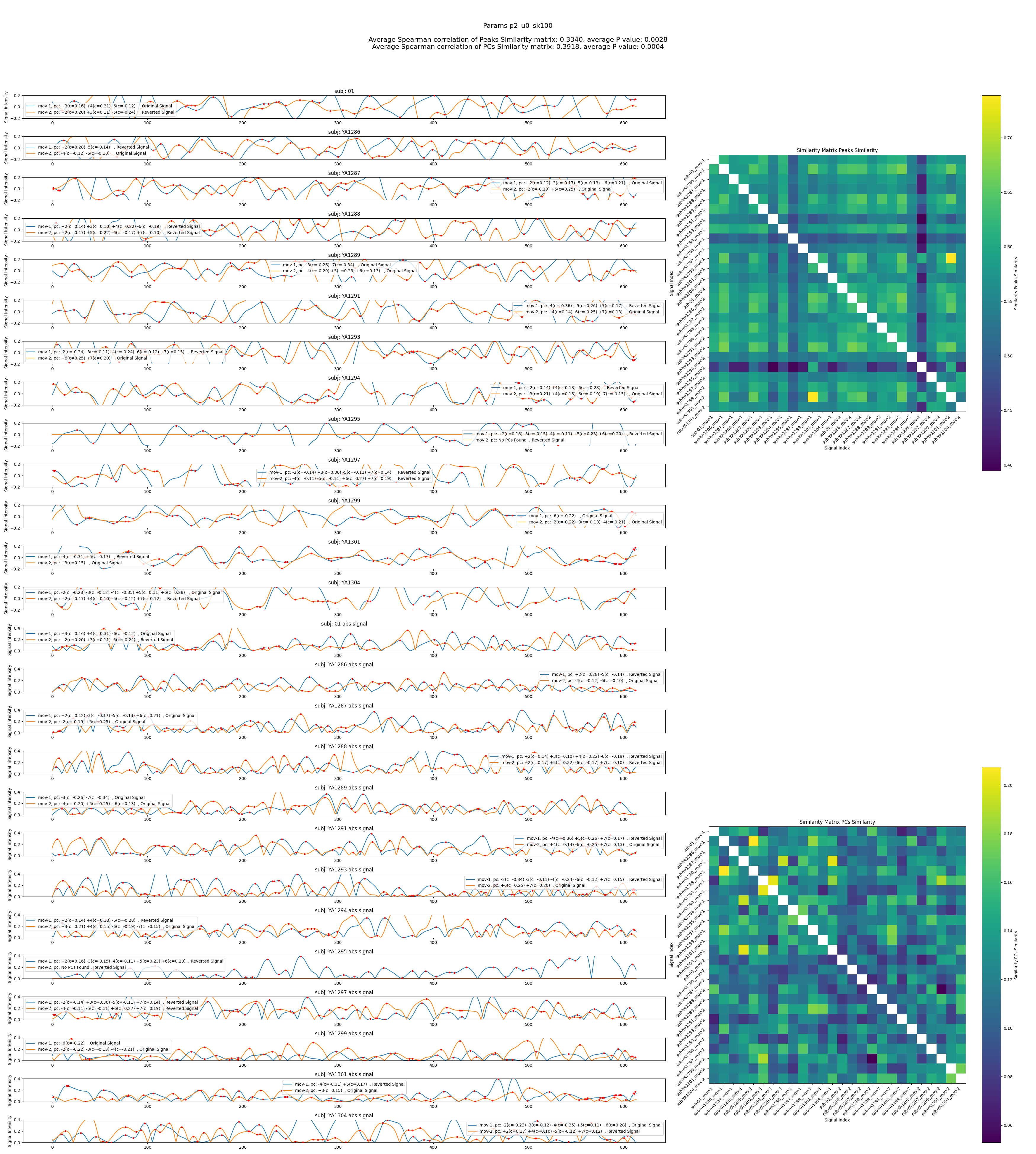
Plot and log
For each combination it saves one figure containing:
Left (signals): for every subject, the reconstructed signal with peak markers, and an “absolute‑value” view beneath it.
Right (heatmaps): a PC‑space similarity matrix and a Peaks‑similarity matrix.
Title: the combination name and the two scores for each matrix.
Keeps “top‑k” best combinations by each score and prints them at the end to the log.
Combine PCs algorithm (used when --combine-pcs is set)
The --combine-pcs mode selects and sums PCs using Pearson correlation
against a movement-specific, windowed (boxcar) regressor.
The procedure is:
Build target regressors (per movement)
Given stimulus times for each movement (
--combine-pcs-stimulus-times), build target regressors that model the expected BOLD response.For each movement, a target regressor is produced either: - Automatically by calling the lag/duration optimizer as described in
find_best_lags.py’s
calculate_lags_durationsfunction;, orFrom user‑supplied lists
--combine-pcs-bold-lag-secondsand--combine-pcs-bold-dur-seconds.
Each regressor is a boxcar (windows of 1.0 across the chosen durations) aligned to
(stimulus_time + bold_lag)and sampled at the subject’s timepoints.
Reconstruct PC time signals
For each subject, compute all PC time signals via:
all_pc_signals = F @ pcs(shapeN × n_components).
Score each PC with Pearson correlation
For every tested PC (except PC0), compute Pearson correlation between the PC signal and the movement’s target regressor.
The absolute correlation (|r|) is used as the match strength.
Select and combine PCs
A PC is considered relevant if
abs(r) > --combine-pcs-correlation-threshold.Relevant PCs are summed into a single combined signal for the subject: - add
+pc_jwhen r > 0 - add-pc_jwhen r < 0For logging, each subject receives a short descriptor like
+pc_1(c=0.32) -pc_3(c=-0.21).
Proceed with peak detection and similarity analysis
The combined signals are used for peak detection and similarity matrix computation as described in steps 5-7 of the main algorithm.
Expected input structure
Root folder (
--files-path) should contain subject folders like:fmri_combinations_results_skfda/ ├── sub-XX_movement1/ │ ├── <param_comb_1>/ │ │ └── eigvecs_eigval_F.npz │ │ └── original_averaged_signal_intensity.txt │ │ └── temporal_profile_pc_0.txt │ │ └── temporal_profile_pc_1.txt │ ├── <param_comb_2>/ │ │ └── eigvecs_eigval_F.npz │ │ └── original_averaged_signal_intensity.txt │ │ └── temporal_profile_pc_0.txt │ │ └── temporal_profile_pc_1.txt │ └── ... ├── sub-XX_movement2/ │ └── ... └── ...
The parameter combination folder names are exactly those created by the sweep script (e.g.,
no_penalty_nb100orp0_u1_t1e-3_l-6_0_nb100).The file it reads per combination is
eigvecs_eigval_F.npz.
Usage
What the Script Does:
Scans the input folder to identify subjects and parameter combinations.
Loads the necessary data files for each subject and parameter combination.
Computes PC similarity and selects representative PCs based on correlations.
Reconstructs time-signals from the selected PCs.
Detects peaks in the reconstructed signals and computes peak similarity matrices.
Calculates consistency scores for both PC and peak similarity matrices.
Generates visualizations and logs the results.
Basic run
compare-pcs \
  --files-path /path/to/fmri_combinations_results_skfda \
  --output-folder /path/to/output_folder
Key options:
--files-path: path containing subject movement folders (see Expected input structure).--output-folder: must NOT exist (it will be created).--movements: movement indices (1..9).--num-scores: number of top parameter combinations to keep.--pc-sim-auto: automatically select representative PC per sample (based on correlations across samples).--pc-sim-auto-best-similar-pc: when used with--pc-sim-auto, count only the single best match from each other file.--pc-sim-auto-weight-similar-pc: exponent applied to absolute correlations when scoring representative PCs.--pc-num-comp: select a specific PC index (starting at 0) for peak comparisons (mutually exclusive with--pc-sim-autoand--combine-pcs).--skip-pc-num: list of PC indices to exclude from analysis.--fix-orientation: attempt orientation correction before peaks comparison.--peaks-abs: compare absolute peak heights (ignore sign).--peaks-dist: minimum distance between detected peaks (default: 5).--skip-timepoints: skip X timepoints at start/end when computing peaks.--combine-pcs: combine PCs based on stimulus timing and BOLD lag (overrides--pc-sim-autoand--pc-num-comp).--combine-pcs-stimulus-times: supply a list of stimulus times per movement; repeat the flag once per movement (action=’append’, default=[]).–combine-pcs-bold-lag-seconds: provide a list of BOLD lag values per movement; repeat this flag once for each movement. If not set, these values are determined automatically (recommended) (action=’append’, default=[]]).
–combine-pcs-bold-dur-seconds: provide a list of BOLD duration values per movement; repeat this flag once for each movement. If not set, these values are determined automatically (recommended) (action=’append’, default=[]]).
--combine-pcs-correlation-threshold: DTW distance threshold for grouping/combining PCs (default: 10.0).--max-workers: 0 = auto (CPU count), 1 = sequential, >1 = parallel worker count.--peaks-all-cpus: If set, use all available CPUs for DTW distance matrix calculation (very fast - appropriate if you use--max-worker 1).
Example command lines (two movements):
Example 1 - use
--pc-sim-auto:
compare-pcs \
  --files-path ` /path/to/fmri_combinations_results_skfda` \
  --output-folder ` /path/to/output_folder` \
  --movements 1 2 \
  --num-scores 10 \
  --pc-sim-auto \
  --pc-sim-auto-best-similar-pc \
  --pc-sim-auto-weight-similar-pc 2 \
  --max-workers 1
Example 2 - use
--pc-num-comp:
compare-pcs \
  --files-path ` /path/to/fmri_combinations_results_skfda` \
  --output-folder ` /path/to/output_folder` \
  --movements 1 2 \
  --num-scores 10 \
  --pc-num-comp 0 \
  --skip-pc-num 3 4 \
  --max-workers 1
Example 3 - use
--combine-pcswith stimulus times and distance threshold, the lags and durations are determined automatically (recommended):
compare-pcs \
  --files-path ` /path/to/fmri_combinations_results_skfda` \
  --output-folder ` /path/to/output_folder` \
  --movements 1 2 \
  --num-scores 10 \
  --combine-pcs \
  --combine-pcs-stimulus-times 30.0 150.75 324.75 360.75 427.5 \
  --combine-pcs-stimulus-times 85.5 228.0 234.75 337.5 \
  --combine-pcs-correlation-threshold 0.1 \
  --max-workers 1
Example 4 - use
--combine-pcswith stimulus times, BOLD lag/duration and correlation threshold:
compare-pcs \
  --files-path ` /path/to/fmri_combinations_results_skfda` \
  --output-folder ` /path/to/output_folder` \
  --movements 1 2 \
  --num-scores 10 \
  --combine-pcs \
  --combine-pcs-stimulus-times 30.0 150.75 324.75 360.75 427.5 \
  --combine-pcs-stimulus-times 85.5 228.0 234.75 337.5 \
  --combine-pcs-bold-lag-seconds -2.0 -3.0 -10.0 -6.0 -8.0 \
  --combine-pcs-bold-lag-seconds -8.0 -13.0 0.0 -13.0 \
  --combine-pcs-bold-dur-seconds 20.0 27.0 20.0 20.0 20.0 \
  --combine-pcs-bold-dur-seconds 17.0 25.0 0.0 25.0 \
  --combine-pcs-correlation-threshold 0.1 \
  --max-workers 1
Notes:
One of
--pc-sim-auto,--pc-num-comp, or--combine-pcsmust be specified.--pc-num-compcannot be used together with--pc-sim-autoor--combine-pcs.--pc-sim-autocannot be used together with--pc-num-compor--combine-pcs.When using
--combine-pcs, the number of repeated--combine-pcs-stimulus-times,--combine-pcs-bold-lag-secondsand--combine-pcs-bold-dur-secondsentries must equal the number of movements.The selection threshold refers to absolute Pearson correlation (range 0..1). Recommended defaults are in the order of
~0.08–0.15depending on data; the command-line option is--combine-pcs-correlation-threshold.If
--combine-pcs-bold-lag-secondsand/or--combine-pcs-bold-dur-secondsare not supplied, lags/durations are computed automatically per movement usingcalculate_lags_durations(seefmri/cli/find_best_lags.py).Ensure the number of repeated
--combine-pcs-stimulus-timesentries matches the number of movements. If lags/durations are supplied, provide them per movement.
Outputs:
The script writes a log file (
compare_peaks_log.txt) and one figure per parameter combination.One figure
similarity_<params>.pngand onesimilarity_<params>.txtper parameter combination:Reconstructed signals and peak markers per subject
Two heatmaps: PC similarity and Peaks similarity
The two consistency scores for each matrix
Example figure showing reconstructed signals and similarity matrices for a parameter combination using parameter --combine-pcs.
Find the best lags and durations around stimulus times - find-best-lags script
The find-best-lags script identifies optimal BOLD response lags and durations around specified stimulus times for fMRI data analysis.
Brief overview
The find-best-lags script searches a results tree (e.g. fmri_combinations_results_skfda),
loads per-PC temporal profiles (temporal_profile_pc_X.txt) and finds the best BOLD
lag and boxcar duration per stimulus event by maximizing mean Pearson correlation
across subjects. It outputs recommendations for each (PC, movement) pair.
Inputs and defaults
Positional:
root_folder— root of the fmri_combinations_results_skfda tree.Optional flags:
--paramsparameter combination folder to analyze (default: p2_u0_sk100)--stimulus-timesexpected stimulus times (in seconds); repeat once per movement (action=’append’, default=[]).--lags-to-testvalues (in seconds) to test for BOLD lag (default: -10..10 s)--durations-to-testtime windows (in seconds) to test for boxcar duration (default: 10..30 s)--pcs-to-testPC indices to analyze - with PC0 excluded (default: 1 2 3 4 5 6)
Outputs
Log file:
find_best_lags_log.txtwritten under the providedroot_folder.Printed and returned recommendations per (PC, movement): best lag, duration, mean correlation, and the final regressor vector.
Usage examples
Minimal invocation:
find-best-lags /path/to/fmri_combinations_results_skfda \
  --params "p2_u0_sk100" \
  --stimulus-times 30.0 150.75 324.75 360.75 427.5 \
  --stimulus-times 85.5 228.0 234.75 337.5 \
Custom search ranges:
find-best-lags /path/to/fmri_combinations_results_skfda \
  --params "p2_u0_sk100" \
  --stimulus-times 30.0 150.75 324.75 360.75 427.5 \
  --stimulus-times 85.5 228.0 234.75 337.5 \
  --lags-to-test -15 -14 -13 -12 -11 -10 -9 -8 -7 -6 -5 -4 -3 -2 -1 0 1 2 3 4 5 6 7 8 9 \
  --durations-to-test 10 11 12 13 14 15 16 17 18 19 20 21 22 23 24 \
  --pcs-to-test 1 2 3
Notes
Repeat
--stimulus-timesonce per movement present in your data.Results are deterministic and saved to the log for reuse.